Equilibrium in Normal Random Movement

In my last post, I touched on my efforts to model how a simple "virus" moves through a population, mainly through the lens of differential equations. As part of that, I wanted to test my model of how the population moves over time. Intuitively, we'd expect the dynamics to follow the Diffusion Equation, which reduces to the Heat Equation if the diffusivity is constant throught the domain.

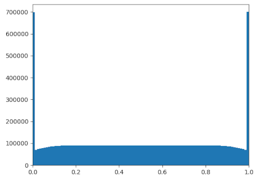Imagine my surprise, then, when I simulated the population to a steady state and got the above distribution. It's inconsistent with the heat equation — we'd be expecting a uniform equilibrium distribution from that. Instead, we get "clumps" on the edges of the simulation domain, as well as "rarefactions" near them.

Granted, the result makes sense. Look at the code that moves people around:

dx = np.random.normal(scale=MOVE_SIGMA, size=(POP_SIZE,))
population += dx
population = np.clip(population, 0.0, 1.0)

A given person has a non-zero probability of winding up exactly on the boundary, unlike everywhere else in the domain. Really, the bounaries are accumulating everyone who overstepped them.

The rarefactions are somewhat harder to explain. The best I can come up with is to compare it to the "unbounded" case. Imagine if the simulation domain streteched to infinity in both directions. Then, with every person moving according to a normal distribution, having a constant population density would be an equilibrium state. When we bound the domain, however, we lose the contribution of everyone outside. This becomes especially noticible near the edges, where almost half of the influx would be coming from outside @@[0,1]@@.

Of couse, I find these "clipping artifacts" undesireable, and I looked for ways to mitigate them. One idea I had was to reroll the positions of people who overstepped instead of simply clipping them to the edge.

dx = np.random.normal(scale=MOVE_SIGMA, size=(POP_SIZE,))
while True:
    population += dx
    outIdx = (population <= 0.0) | (population >= 1.0)
    numOut = np.sum(outIdx)
    if numOut != 0:
        population[outIdx] -= dx[outIdx]
        dx[~outIdx] = 0.0
        dx[outIdx] = np.random.normal(scale=MOVE_SIGMA, size=(numOut,))
    else:
        break

This did get rid of the people clumped to the edge, but it still left the rarefactions. In fact, it actually made them much worse.

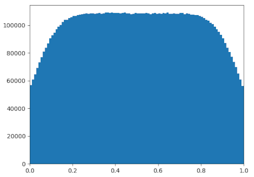
On a side note, decreasing the variance for people's movement seemed to help significantly. In my simulation, all the people moved according to a normal distribution, and the above figures were collected with @@\texttt{MOVE_SIGMA} = \sigma = 0.1@@. This value can be made arbitrarily small — if, every second, people move according to a normal distribution with variance @@\sigma^2@@, simply do @@n@@ "runs" with variance @@\frac{1}{n}\sigma^2@@ to simulate one second, where @@n@@ can be made arbitrarily large.

That works in theory, but not in practice. If we have a population of size @@\texttt{POP_SIZE} = K@@ and we simulate for @@t@@ seconds, then simulating takes @@\mathcal{O}(ntK)@@ time. That's not great, especially since two of those parameters are being made really large. However, we only really want to see the equilibrium state for now, and it might be better to calculate it rather than to simulate it out.

To do this, we can start by formalizing the problem we are trying to solve. I'll consider the case where we clip the people to the edges of the domain, and the case where we reroll can be built on top of it. We can specify the state of our system with a number @@\rho_{\text{side}}@@, specifying the proportion of people clipped to one side, as well as a function @@\rho: [0,1] \to \mathbb{R}^+@@, specifying the density of people at a particular location. The system proceeds by computing %%\begin{align*} \rho_{\text{side}} &:= \frac{\rho_{\text{side}}}{2} + \frac{\rho_{\text{side}}}{\sqrt{2\pi\sigma^2}} \int_{-\infty}^{-1} e^{-\frac{t^2}{2\sigma^2}}\,dt + \int_0^1 \int_{-\infty}^{0} \frac{\rho(x)}{\sqrt{2\pi\sigma^2}} e^{-\frac{(t-x)^2}{2\sigma^2}} \, dt \, dx \nl \rho(x) &:= \frac{\rho_{\text{side}}}{\sqrt{2\pi\sigma^2}} e^{-\frac{x^2}{2\sigma^2}} + \frac{\rho_{\text{side}}}{\sqrt{2\pi\sigma^2}} e^{-\frac{(x-1)^2}{2\sigma^2}} + \int_0^1 \frac{\rho(t)}{\sqrt{2\pi\sigma^2}}e^{\frac{(x-t)^2}{2\sigma^2}} \, dt . \end{align*}%% The first term is the contribution from the left "wall", the second term that from the right wall, and the third term that from everywhere else. This iteration is quite complicated, and I highly doubt there is a closed form expression for the fixed points.

So, we approximate. We can discretize the domain into @@\texttt{NUM_BINS} = N@@ regions of equal length @@\texttt{BIN_DELTA} = \Delta@@, treating the two walls separately, and create a Markov matrix @@\texttt{markovMat} = \mathbf{M}@@ for movement between the regions. For calculation, we'll say that the population density is constant throught a given region. As for indexing, let index @@0@@ be the left wall, index @@N+1@@ the right wall, and each of the "bins" indexed left to right starting at @@1@@. Also, we'll use left stochastic matrices because that's what numpy seems to play better with — @@M_{j,i}@@ represents the probability of transitioning to state @@j@@ given you are in state @@i@@.

We can then go through the caclulations. First, we take care of transitioning between walls: %%\begin{align*} M_{0,0} = M_{N+1,N+1} &= \frac{1}{2} \nl M_{N+1,0} = M_{0,N+1} &= \frac{1}{\sqrt{2\pi\sigma^2}} \int_{-\infty}^{-1} e^{-\frac{t^2}{2\sigma^2}} \, dt. \end{align*}%% Now, consider transitioning between a wall and a bin @@B@@, and vice versa: %%\begin{align*} M_{B,0} = M_{N+1-B,N+1} &= \frac{1}{\sqrt{2\pi\sigma^2}} \int_{(B-1)\Delta}^{B\Delta} e^{-\frac{t^2}{2\sigma^2}} \, dt\nl M_{0,B} = M_{N+1,N+1-B} &= \frac{1}{\sqrt{2\pi\sigma^2}} \int_{(B-1)\Delta}^{B\Delta} \int_{-\infty}^0 e^{-\frac{(t-x)^2}{2\sigma^2}} \, dt \, dx. \end{align*}%% Finally, consider transitioning from a bin @@b@@ to another bin @@B@@: %% M_{B,b} = \frac{1}{\sqrt{2\pi\sigma^2}} \int_{(b-1)\Delta}^{b\Delta} \int_{(B-1)\Delta}^{B\Delta} e^{-\frac{(t-x)^2}{2\sigma^2}} \, dt \, dx. %%

The above formulas aren't nice. Far from it. But, they are computable. We can even get a "closed-form" solution using the error function @@\text{erf}@@, implemented in Python as math.erf. We can use the formulas above to populate @@\mathbf{M}@@, from where we can solve for an eigenvector with eigenvalue one by computing @@(\mathbf{M} - \mathbf{I})\mathbf{v} = \mathbf{0}@@. In fact, since @@\texttt{solMat} = \mathbf{M} - \mathbf{I}@@ is not full rank, we can replace one of the rows with another constraint to get a particular @@\mathbf{v}@@. For instance, I required the numbers in the vector to sum to a particular value, corresponding to a fixed population size.

solMat[-1] = np.ones((markovMatSize,))
solVec[-1] = POP_SIZE
sol = np.linalg.solve(solMat, solVec)

This algorithm is @@\mathcal{O}(N^3)@@, which was much faster than simulating for me. It was just a question of how well it worked.

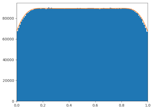It worked pretty well. The above figure is the output of the Markov chain (in orange) compared to simulating until equilibrium (in blue). It was done with clipping, with @@\sigma = 0.1@@, and with @@N = 100@@. The outputs inside the simulation domain are fairly close, and numbers of people clipped (not shown on the graph above to avoid clutter) differ by only @@0.3\%@@.

What I've said so far only applies to the case where we clip people to the boundaries. Thankfully, rerolls are just a small extension to this. We simply compute @@\mathbf{M}@@ as described above, neglect the cases where a person goes into or comes out of a "wall," then renormalize all the probabilities to sum to one.

markovMat = np.delete(markovMat, [0,-1], axis=0)
markovMat = np.delete(markovMat, [0,-1], axis=1)
markovMat /= np.sum(markovMat, axis=0)

Again, it works fairly well. Of course, my work here is far from perfect, and there's probably still a lot more that can be done to refine the model. For instance, you might notice that the Markov chain seems to overestimate the number of people around the edges. Why is that? I invite you all to take a look at the code and see what you can find.

Resources

• Code for this post